Winning with the Bear: GEM strategies comparison
Introduction
Momentum based strategies work well in up-trending markets. Fit a curve to the price data, rank tokens by the quality and strength of their trend, select a portfolio of winners. In a bull market, there are plenty of winners to choose from.
But what happens in a bear market?
- the winners are few and apart
- the rare upwards trends are short-lived
The 2022 is but the most textbook example of a crypto bear market – especially the period from May through December, when BTC had already fallen 50% from its all-time high, Luna had collapsed, and the market was unambiguously grinding down. I ran a series of experiments on historical data, trying to gauge whether a simpler linear model can be more responsive to the short upward trends as compared to a compounding curve.
TL;DR The choice of regression model turns out to be almost irrelevant, what matters the most seems to be the length of the fitting window.
The GEM Pipeline
The GEM pipeline fits a regression model to each token’s daily closing prices, then selects a portfolio based on the fit quality and trend strength.
For each token on each day:
- Fit: Normalize timestamps to sequential day indices (0, 1, 2, …) and fit a trend model to the closing prices
- Evaluate: Compute R-squared and a momentum score
- Filter: Keep tokens with positive trend, R-squared above a threshold, and the momentum below a cap (to exclude pump-and-dump spikes)
- Weight: Rank by momentum, take the top N, and assign inverse-volatility weights using Average True Range (ATR). This is the portfolio.
The baseline model uses a two-step exponential regression:
\[y = a_0 \cdot a_1^{x}\]First, a log-linear OLS fit ($\ln y = b_0 + b_1 x$) provides initial parameter estimates. These are refined via Levenberg-Marquardt optimization into the exponential form. Momentum is then $R^{2} \cdot (a_1 - 1) \cdot 100$, where the R-squared exponent controls how much low-quality fits are penalized.
The experimental linear model fits directly in price-space:
\[y = b_0 + b_1 \cdot x\]Momentum becomes $R^{2} \cdot (b_1 / \bar{p}) \cdot 100$, where $b_1 / \bar{p}$ normalizes the slope by the mean price to produce a percentage daily trend, analogous to $a_1 - 1$ in the exponential case.
The rest of the pipeline – ATR computation, portfolio construction, differential rebalancing, and cooldown – is identical between the two models.
Experiment Setup
Window: May 1 – December 31, 2022. By May, BTC had already dropped roughly 50% from its November 2021 ATH. The Luna collapse (May 9), 3AC liquidation (June), and FTX collapse (November) all fall within this window. No doubt the bear is already here.
Token universe: A curated “bear portfolio” of safe-haven assets available on Binance:
| Token | Type | Coverage |
|---|---|---|
| PAXGUSDT | Tokenized gold | Full (May–Dec, 245 candles) |
| EURUSDT | EUR stablecoin | Full (May–Dec, 245 candles) |
| USDCUSDT | USD stablecoin | Partial (May–Sep, 149 candles) |
| TUSDUSDT | USD stablecoin | Partial (May–Sep, 149 candles) |
Models and their parameter configs:
We use the so called “bear” and a “ranging” specialist models, GEM models with their parameters selected towards capital preservation and cautious exploration of the token universe, respectively:
| Bear | Ranging | |
|---|---|---|
| top_n | 1 | 8 |
| R-squared threshold | 0.5 | 0.3 |
| Rebalance cooldown | 10 days | 5 days |
| Momentum cap | 0.14 | 0.20 |
| R-squared exponent | 2.0 | 1.5 |
Fee model: We assume 0.3% per trade (0.10% exchange fee + 0.20% slippage estimate).
Benchmark: Equal-weight buy-and-hold across all four tokens. This is what we want to beat.
First Attempt: Full History Fitting
First run used the standard GEM approach: fit the regression model to all available history from the start of the window up to the current day. On day 100, the model sees all 100 preceding candles.
The results:
| Strategy | Return | Max Drawdown | Sharpe |
|---|---|---|---|
| Exp GEM, bear params | 0.00% | 0.00% | 0.00 |
| Lin GEM, bear params | 0.00% | 0.00% | 0.00 |
| Buy & Hold | -0.65% | -6.01% | -0.12 |
| Exp GEM, ranging params | -4.01% | -4.21% | -1.91 |
| Lin GEM, ranging params | -4.01% | -4.21% | -1.91 |
The bear specialist didn’t trade at all, it sat in cash for the entire eight months - winning on capital preservation.
At the same time it failed to capture any of the intermediate rallies that occurred during this period. PAXG, for instance, rallied roughly 10% from its June lows through August as gold spiked during the 3AC liquidation chaos.
To understand why, we examined what the models actually computed on several randomly sampled dates:
| Date | Token | Model | a1 | R-squared | Growth filter |
|---|---|---|---|---|---|
| 2022-08-01 | PAXGUSDT | exp | 0.9990 | 0.68 | FAIL |
| 2022-08-01 | PAXGUSDT | lin | 0.9990 | 0.69 | FAIL |
| 2022-08-01 | EURUSDT | exp | 0.9995 | 0.52 | FAIL |
| 2022-10-15 | PAXGUSDT | exp | 0.9992 | 0.82 | FAIL |
Every token, on every date, had a growth parameter below 1.0 (negative overall slope). The R-squared was often strong – meaning the model was confidently fitting a downtrend. But the growth filter ($a_1 > 1$) rejected everything, because the cumulative history from May 1 was dominated by the initial hard crash.
The ranging specialist, with its looser R-squared threshold (0.3), did enter positions – and promptly lost money, because it was catching the tail end of downtrends, not rallies.
The core problem: fitting over the entire history anchors the model to the dominant long-term bear trend. The exponential model compounds this: it assumes multiplicative growth, making it even harder for a short 2-week price rally to overcome the long negative history.
Rolling Window
The solution is to limit the regression to a rolling window of recent data.
This reframes the model from a cumulative trend detector to a short-term momentum detector, catching the short-lived rallies.
R-squared plays a dual role in this setup:
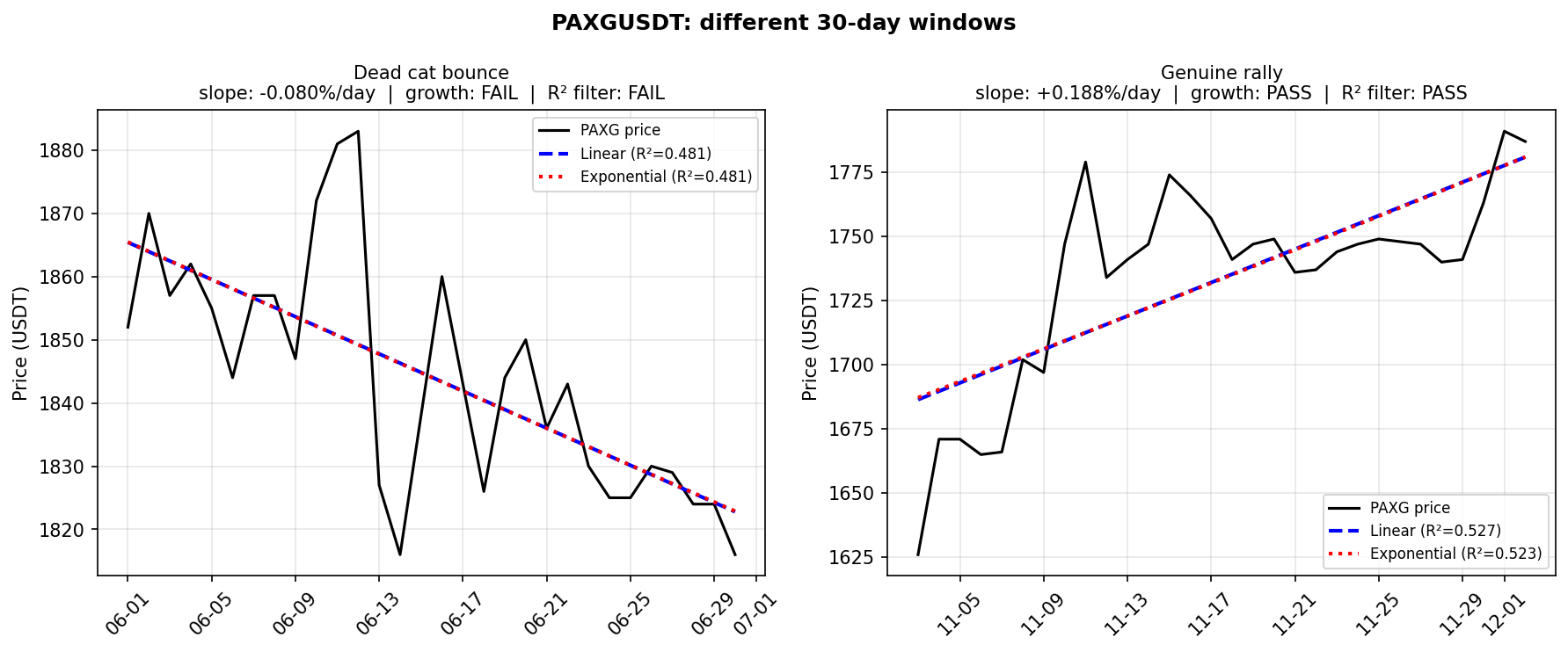
- A genuine rally over a 30-day window produces a clean uptrend and high R-squared
- A “dead cat bounce” is noisy and V-shaped – the linear fit is poor, R-squared is low, and the position gets filtered out
I tested three window sizes – 15, 30, and 60 days – across both models and both parameter configs:
| Config | Return | Max DD | Sharpe | Sortino | Calmar | Rebalances |
|---|---|---|---|---|---|---|
| bear-w30 | +6.40% | -1.39% | 1.59 | 3.33 | 6.98 | 21 |
| bear-w60 | +3.77% | -1.10% | 1.13 | 2.34 | 5.14 | 19 |
| Buy & Hold | -0.65% | -6.01% | -0.12 | -0.17 | -0.16 | 0 |
| ranging-w30 | -0.28% | -9.42% | -0.02 | -0.03 | -0.04 | 29 |
| ranging-w60 | -1.02% | -5.30% | -0.27 | -0.40 | -0.29 | 37 |
| bear-w15 | -6.27% | -8.77% | -1.46 | -2.09 | -1.05 | 24 |
| ranging-w15 | -9.28% | -10.42% | -1.94 | -2.51 | -1.30 | 45 |
Three observations stand out:
1. The 30-day window seems to be the sweet spot. It captures the PAXG (gold) summer rally: long enough for R-squared to recognize a genuine consistent trend, short enough to not get anchored by the preceding months of decline. The 15-day window is too reactive – it enters and exits on noise, bleeding fees across 24+ rebalances. The 60-day window is too slow – it captures the rally, but enters late and exits late, leaving profits on the table.
2. Bear params (top_n=1) dominate ranging params (top_n=8). In a 4-token safe-haven universe, concentrating on the single best opportunity outperforms diversification.
3. The exponential and linear based GEM models produced almost identical results at every window size. The choice of regression model is irrelevant.
What the Winner Holds
This is how the bear-w30 model earns its return – every rebalance event over the 8-month window:
| Day | Date | Action | Holding | Momentum | R-squared | Value |
|---|---|---|---|---|---|---|
| 0 | 2022-05-01 | TO CASH | CASH | $10,000 | ||
| 10 | 2022-05-11 | TO CASH | CASH | $10,000 | ||
| … | … | TO CASH | CASH | $10,000 | ||
| 162 | 2022-10-10 | TO CASH | CASH | $10,000 | ||
| 192 | 2022-11-09 | ENTER | EURUSDT | 0.022 | 0.50 | $9,970 |
| 202 | 2022-11-19 | HOLD | EURUSDT | 0.087 | 0.68 | $10,341 |
| 212 | 2022-11-29 | HOLD | EURUSDT | 0.118 | 0.75 | $10,313 |
| 222 | 2022-12-09 | HOLD | EURUSDT | 0.044 | 0.71 | $10,525 |
| 232 | 2022-12-19 | ROTATE | PAXGUSDT | 0.086 | 0.79 | $10,539 |
| 242 | 2022-12-29 | ROTATE | EURUSDT | 0.029 | 0.70 | $10,575 |
Model kept patiently for six and a half months of in all cash, then entered into a clean trend:
- From May through October, every rebalance evaluates candidates and finds nothing.
- No token sustains a positive 30-day slope with R-squared above 0.5 and the model (correctly) stays out of the market.
- On November 9, the EUR begins a sustained rally against the dollar.
- The 30-day window picks up a clean uptrend – R-squared just clears 0.50 – and the model enters EURUSDT.
- Over the next 6 weeks, the trend strengthens: R-squared climbs to 0.75, momentum rises, and the portfolio value grows to $10,525.
- On December 19, PAXG briefly shows a stronger trend (R-squared 0.79) and the model rotates for one brief period before returning to EUR.
- The strategy finishes at $10,640 – a 6.40% return in a period where BTC fell 65% from ATH and the equal-weight buy-and-hold benchmark lost 0.65%.
It waits for a trend that passes strict quality filters, then concentrates its entire portfolio on that single opportunity.
Next Steps
The above results come from a hand-curated 4-token safe-haven portfolio. The natural folow-up question is: what happens when we run the same experiment on the full Binance token universe?
With hundreds of tokens, the model has a much richer candidate pool on each rebalance day. Does it converge to the same safe-haven tokens (PAXG, EUR) that we hand-picked, or does it find opportunities we didn’t anticipate?
The full universe also gives the exponential and linear models a chance to diverge on the more volatile altcoin data.