Aggressive bear: GEM shorting in downwards markets
Introduction
In a previous post we looked at GEM market bear models, who can show a win even in a market in a adverse conditions. The bear specialist GEM model won by mostly not playing. It sat in cash for six and a half months of 2022, then entered EURUSDT once a clean uptrend emerged – with a brief rotation through PAXG (tokenized gold) in late December – finishing the window at +6.40% while BTC was down roughly 65% from its all-time high.
In this post we research a different, more aggressive strategy. Instead of a safe haven of tokens, we look at a broader spectrum. We invert the GEM filters, weight by the magnitude of the negative trend, and short the weakest tokens on Binance USDⓈ-M perps.
TL;DR
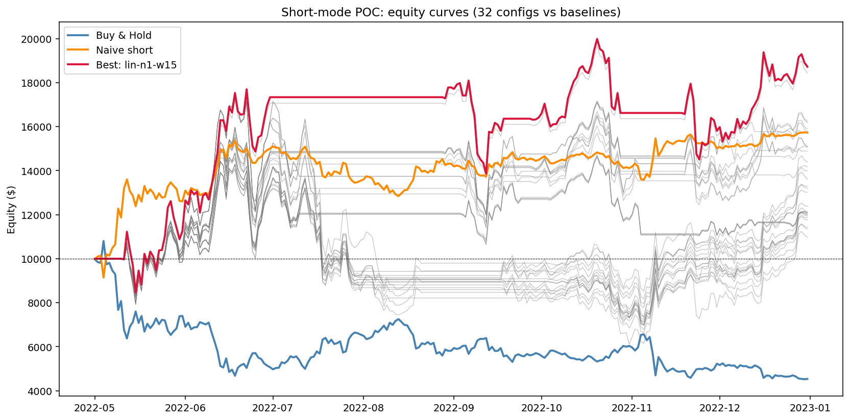
On an 11-token mixed bear-market universe, the best aggressive short-mode GEM config (lin-n1-w15) returns +87.2% over May–Dec 2022 with a -27.4% drawdown, for a Calmar of 5.64 – beating the long-only bear specialist’s Calmar 4.6.
Yet it loses on Calmar to a naive equal-weight short of the same universe (+57.72% returns, -16.41% max drawdown, Calmar 5.92). The single most meaningful drawdown comes from an ADA short squeeze - something that a model looking just at the daily candles cannot see coming.
From defense to offense
The bear specialist was long-only and held a single token at a time. The aggressive variant inherits the GEM ranking core, with the adjustments below.
Short mechanics on USDⓈ-M perps. A position is $(\text{quantity}, \text{entry_price})$. PnL on close is $\text{quantity} \times (\text{entry_price} - \text{exit_price})$ – gains when the price falls. Funding is paid (or received) every 8 hours; in a bear market with crowded shorts, funding is usually slightly negative for shorts, so the position accrues a small penalty each settlement. Aggregated to daily, mean funding rates over the window ranged from roughly -5% to -30% annualised across tokens.
Sign-flipped filters. The GEM core rejects positive $a_1$ candidates and requires $\text{momentum} < -\text{momentum_floor}$. The exponential model also wants $a_1 < 1$ (a compounding decline); the linear model wants a negative normalised slope. R-squared and ATR play the same roles as in the bull/bear long specialist models.
Momentum-magnitude weighting. The previous specialists weighted by inverse ATR – resulting in less exposure to the more volatile assets. For an aggressive short, we want the opposite: the strongest negative trend deserves the largest allocation. Weights are $|m_i| / \sum_{j} |m_j|$ over the top $N$ picks.
The rest – fitting window, R-squared threshold, differential rebalancing, cooldown – is identical to the bear specialist.
Experiment Setup
Window: Same May 1 – December 31, 2022 window as previously: BTC already down ~50% from ATH, Luna collapsed (May 9), 3AC liquidated (June), FTX collapsed (November). Unambiguously a bear market.
Universe: 11 Binance USDⓈ-M perpetuals, deliberately mixing fallers and outperformers over the period, such that the selector has a discrimination problem to solve.
| Group | Tokens | End-of-window return |
|---|---|---|
| Extreme fallers | SOL, AVAX, ADA, DOT | -69% to -89% |
| Moderate fallers | BTC, ETH, LINK, MATIC | -31% to -58% |
| Outperformers | BNB, TRX, XMR | -23% to -37% |
The outperformers are the controls: a working momentum selector should not waste capital shorting them when fallers are available.
Data: daily klines and 8-hour funding history from Binance. $10,000 starting capital, 0.3% round-trip fee, 10-day rebalance cooldown.
Sweep: 32 configurations.
\[\text{fit_window} \in \{15, 30, 60, 90\} \quad\times\quad \text{top_n} \in \{1, 3, 5, 8\} \quad\times\quad \text{model} \in \{\text{exp}, \text{lin}\}\]Experiment verdict structure: Three stages, each PASS / NO-PASS:
- Stage 1: best-config Calmar > naive equal-weight short Calmar
- Stage 2: best-config Calmar > long-only bear specialist (Calmar 4.6 from the previous post)
- Stage 3: robust across configs ($\geq$ 1/3 positive Calmar AND a dominant
fit_windowin the top 6 models)
Sweep Results
Top of the 32-config sweep, sorted by Calmar:
| Config | Return | Max DD | Calmar | Sharpe | Rebalances |
|---|---|---|---|---|---|
| lin-n1-w15 | +87.2% | -27.4% | 5.64 | 1.39 | 22 |
| exp-n1-w15 | +84.3% | -27.4% | 5.42 | 1.36 | 22 |
| exp-n8-w15 | +62.5% | -24.6% | 4.31 | 1.23 | 22 |
| lin-n8-w15 | +61.8% | -24.6% | 4.26 | 1.22 | 22 |
| exp-n5-w15 | +58.9% | -24.9% | 3.99 | 1.15 | 22 |
| lin-n5-w15 | +57.7% | -24.9% | 3.90 | 1.14 | 22 |
| lin-n3-w30 | +50.4% | -25.6% | 3.27 | 1.01 | 21 |
| lin-n3-w15 | +51.0% | -27.0% | 3.14 | 1.02 | 22 |
Three observations, mirroring the bear-long specialist’s findings:
1. fit_window=15 dominates the top quartile.
All top six configs share w=15.
Tight windows track the bear’s punctuated drawdowns; wider windows (60, 90) catch the intermittent relief rallies and the max drawdown blows out to ~50% (data not included, we refer to the notebook).
Similar finding as in the previous post: the bear-long specialist preferred w=30.
2. Concentration outperforms diversification on this universe.
top_n=1 produces the highest return (+87%) and Calmar (5.64).
top_n=8 reduces both return (+62%) and DD (-24.6%), but the Calmar drops to 4.31.
With only 7 real fallers in the universe, diluting into 5 or 8 names forces the selector to short weaker signals alongside the strongest, and that costs more in return than it saves in drawdown.
The token universe is however probably too small to draw any larger conclusions from this fact.
The naive model winning on overall Calmar is due to the risk diversification.
3. The choice of regression model is, again, irrelevant.
lin-n1-w15 and exp-n1-w15 are within 0.2 Calmar of each other.
Same pattern as the previous post: the fitting window dominates the model family.
What the winner does
The best config holds a single token at a time, rebalances every 10 days when momentum changes hands, and goes to cash when no token clears the entry threshold.
Twenty-two rebalances over 245 days. The equity story splits into two phases:
| Phase | Days | Equity move |
|---|---|---|
| Capture | 10 → 60 (May 11 – Jun 30) | $10,000 → $17,338 (+73%) |
| Survive | 60 → 242 | $17,338 → $19,291 (+11%) |
Most of the gains happen in the first seven weeks. The model catches SOL → AVAX → SOL → BNB → ETH in the May–June crash, rides each for 10 days, and exits to cash on June 30 when the momentum-cross trigger fires. It then sits in cash for sixty days through July and August – the bear-market relief rally that wiped out anyone holding shorts through the chop – and re-engages in late August.
The strategy is “catch the trend, then survive the chop.” About 30% of the window is spent in cash.
The most-shorted name was SOL at 17.6% of the window, followed by ETH, ADA, and BNB at ~8% each.
The short squeeze problem
The single meaningful drawdown comes from an ADA short squeeze.
On October 8 the model shorted ADA which at that time had a clean, 15-day downtrend. On October 18 the trend was even cleaner; momentum-magnitude weighting kept ADA at 100% of the book. On October 28 ADA was up roughly 15% from the Oct-18 reentry. The peak equity at Oct 18 was $18,817; by Oct 28 it was $16,622. ~12% drawdown in ten days, on one position.
But than what happened is a textbook short squeeze: a token already down 70% from its highs, heavily shorted (funding rates flipped to “shorts pay longs” in the days before), price ricocheting back from $0.30s to $0.40 as overcrowded shorts got liquidated, forcing even more buying.
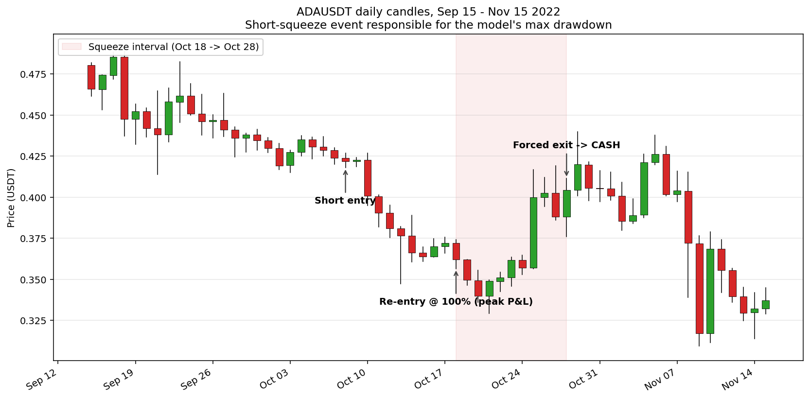
Daily OHLCV cannot anticipate this. The price trend was clean and negative – exactly what the model is built to detect. The information that would have flagged the risk – funding rate inversion, open interest divergence, liquidation cluster proximity – is not in the kline feed.
This is the meta-finding the post is about: the model’s risk is mostly squeeze risk, and the information lives outside just the price data.
Baselines and the Stage Report
The two reference strategies on the same universe:
| Strategy | Return | Max DD | Calmar | Sharpe |
|---|---|---|---|---|
| Buy & Hold (11-token equal weight) | -54.5% | -58.1% | -1.19 | -0.85 |
| Naive equal-weight short, no rebalance | +57.7% | -16.4% | 5.92 | 1.48 |
| GEM short, lin-n1-w15 | +87.2% | -27.4% | 5.64 | 1.39 |
| Long-only bear specialist (previous post) | n/a | n/a | 4.60 | 1.59 |
Stage Report:
| Stage | Criterion | Result |
|---|---|---|
| Stage 1 | best Calmar > naive Calmar | NO-PASS (5.64 vs 5.92, $\Delta$ -0.28) |
| Stage 2 | best Calmar > long-only bear (4.6) | PASS ($\Delta$ +1.04) |
| Stage 3a | $\geq$ 1/3 configs positive Calmar | PASS (32/32) |
| Stage 3b | dominant fit_window in top 6 |
PASS (w15, 6/6) |
The Stage 1 NO-PASS deserves comment, because it would be easy to read it as “the model adds nothing over a naive baseline.”, but that is not what is happening.
The naive equal-weight short holds 11 tokens equally, all the way through.
Its max drawdown is structurally smaller than any 1-asset short can match – the diversification across 11 names naturally limits the impact from DD events – at the cost of lower returns (+57.7% vs +87.2%).
The GEM short with top_n=1 is, by construction, more exposed to token event risks (see short squeeze).
Stage 2 confirms the signal is there: the model clears the long-only bear specialist, despite carrying the big drawdown event. Stage 3 confirms the signal is clustered, not a single-config artifact: all top 6 configs share the same fit window, and 32 of 32 configurations produce positive Calmar.
Verdict: the signal is real but marginal
The headline number is good but the universe is too small to know if the strategy generalises.
At top_n=1 the model is a “find the biggest faller” oracle and pays the concentration cost.
At top_n=5 and top_n=8 it dilutes into weaker signals – but only because there are only seven real fallers in the universe to begin with.
A 25–35 token universe with the same top_n=5 or top_n=8 could more than likely let the diversification do its work without forcing the selector to short noise.
Defences against squeezes
Daily OHLCV cannot see ADA-style snap-backs coming. The model needs information from outside the kline feed.
CoinGlass or e.g. Hyblock offer (paid) liquidation heatmaps, but the sam esignal can be hand-built. Below are some ideas:
1. Per-token concentration cap + trailing stop. Cap any single short at 8–10% of NAV. Apply a 15–20% trailing stop from the entry-adjusted peak P&L. Pure portfolio logic, no new data pipeline. This cheap defense alone would have capped the ADA hit at roughly half of its actual DD cost.
2. Funding rate signal. Binance, Bybit or OKX all publish funding-rate history (already used in the experiment to calculate per-position cost accrual). Potential heuristic: if funding crosses above +0.05% for three consecutive periods on an asset we are short, halve the position, if it crosses +0.1%, exit the position. A crowded-short detector.
3. Intraday volume-spike + reversal exit. If a shorted name prints $\ge 3 \cdot \sigma$ volume on a green candle that reclaims the prior day’s high, exit at next bar. Requires 1h or 15m kline ingestion.
Together these cover most of what a paid liquidation-heatmap API service would.
Next Steps
Capital preservation as a strategy works – the previous post showed that. Aggressive shorting works too, with caveats – as the results of this brief experiment have shown. An interesting question is what happens when the regime detector decides how much of each to deploy.
Below some ideas:
-
Wider universe: All Binance USDⓈ-M majors that existed in May 2022. See if diversified models start to prevail.
-
Squeeze defenses: Add the funding+OI composite score and a trailing stop rules. Akin to liquidation heatmaps. Rerun the same sweep with the defenses on. If the ADA-shaped drawdown shrinks meaningfully without killing the returns, the defenses earn the keep.
-
Regime-weighted composition: connect the specialists (bull, rangin, bear-long, bear-short) to the HMM regime probabilities. Bear sub-specialist models could be blended using a tuned parameter - learned on the historical regime exposure.